BigSort: Sorting TBs of Data with GBs of RAM
Concept. BigSort is external merge-sort. It sorts a table larger than RAM by reading RAM-sized chunks, sorting each chunk in memory, writing them back to disk, then merging the sorted chunks together.
Intuition. When you need to sort a 64 GB Listens table by rating on a 6.4 GB machine, read 6.4 GB at a time, sort each chunk in RAM, write each sorted chunk back, then merge the 10 sorted chunks. Cost: read every page once, write every page once, per pass.
Interactive BigSort Animation
Watch BigSort in Action
The BigSort Algorithm (aka External Sort)
Core Idea
-
Divide: Create sorted runs that fit in memory.
-
Conquer: Merge those sorted runs into your final output.
ALGORITHM: BigSort
BigSort(file, B):    // B = total RAM pages available

    // Phase 1: Create sorted runs
    runs = []
    while not EOF:
        chunk = read(B pages)
        sort(chunk)           // quicksort in RAM
        write(chunk to run_i)
        runs.add(run_i)

    // Phase 2: Merge runs
    while |runs| > 1:
        next_runs = []
        for i = 0 to |runs| step B-1:
            batch = runs[i : i+B-1]   // B-1 input buffers + 1 output buffer
            merged = KWayMerge(batch)
            next_runs.add(merged)
        runs = next_runs
    return runs[0]

Result: Fully sorted file
Cost: C_r×N + C_w×N per pass
Key Property: Handles any file size with limited RAM
Why Sort?
Sorting is the backbone of a database. Every ORDER BY, every range scan on a B+Tree, every sort-merge join, every LSM compaction starts here. PostgreSQL, BigQuery, Spark all run the same operation underneath. Get sort right and the rest of the engine gets fast.
Example Problem: Break Big Sort Into Small Sorts
64GB
Unsorted Table
6.4GB
Available RAM
10×
Size Mismatch
BigSort
The Solution
SOLUTION. Apply BigSort to this 10× mismatch: split into 10 sorted runs of 6.4 GB each (Phase 1), then a single 10-way merge with 9 input buffers and 1 output buffer produces the fully sorted 64 GB file (Phase 2). Single merge pass, so cost is 4N IOs total.
Cost Analysis
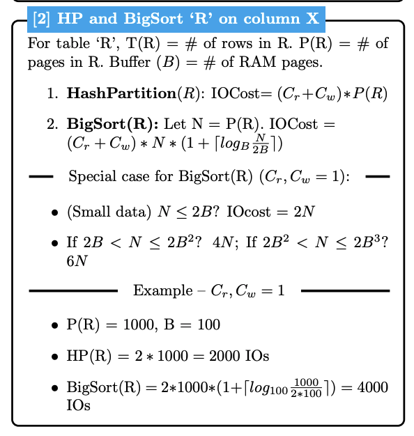
For detailed IO cost formulas, see IO Cost Reference.
BigSort vs Hash Partitioning: Cost Intuition
Hash Partitioning: Always 2N IOs
-
Single pass through data, read once, write once to partitions.
-
Cost stays constant regardless of data size.
BigSort: Variable cost, grows logarithmically
-
Multiple passes needed as data gets bigger.
-
More data means more sorted runs, which means more merge passes required.
-
Small data (fits in few runs): ~4N IOs.
-
Large data (many runs): ~6N, 8N, 10N IOs...
Why the difference? Hash Partitioning distributes data in one shot, but BigSort must repeatedly merge until everything is sorted.
Key Takeaways
-
Divide and Conquer: Split large sorts into small sorts, then merge. Sort TB of data with GB of RAM.
-
Scalable Cost: Works for any big data size with fixed RAM.
-
Foundation of Big Data: This is how PostgreSQL, BigQuery, and Spark handle
ORDER BY.
Next
Block Nested Loop Join → Joining two big tables is the first algorithm that combines everything so far: row access, RAM-sized blocks, and repeated scans.