IO Cost Summary: Comparing Query Plans

Concept. The IO cost of a query plan is the sum of the IO costs of every step in the plan. To compare plans, you add up each step's cost using the formulas for sort, hash partition, and the three join algorithms.

Intuition. Two plans that produce the same result can cost wildly different amounts of IO depending on which algorithm you use at each step. This page walks through one recommendation query and computes the total cost of two plausible plans side by side.

The cost formulas used here (BigSort, HP, and the three joins BNLJ / SMJ / HPJ, all in terms of C_r, C_w, and page counts P(...)) are the ones defined in Module 3 nanoDB: IO Algorithms. This page does not introduce new formulas; it adds them up across a plan.

The Query

-- Highly recommended songs
SELECT r.song_id, COUNT(r.recommendation_id) AS recommendation_count
FROM Recommendations AS r
JOIN Listens AS l ON r.user_id = l.user_id AND r.song_id = l.song_id
GROUP BY r.song_id
ORDER BY COUNT(r.recommendation_id) DESC;

The Recommendations table. Alongside the canonical Users / Songs / Listens schema, the recommender writes one row per song it suggests to a user: Recommendations(user_id, song_id, recommendation_id, recommendation_time), with user_id and song_id foreign keys into Users and Songs. The query joins it to Listens on the pair (user_id, song_id), so a match means "this user actually listened to a song that was recommended to them."

Three goals to achieve in any plan: JOIN the two tables on (user_id, song_id), GROUP BY song_id, then SORT by count.

Query Plan #1: Sort-Merge Join

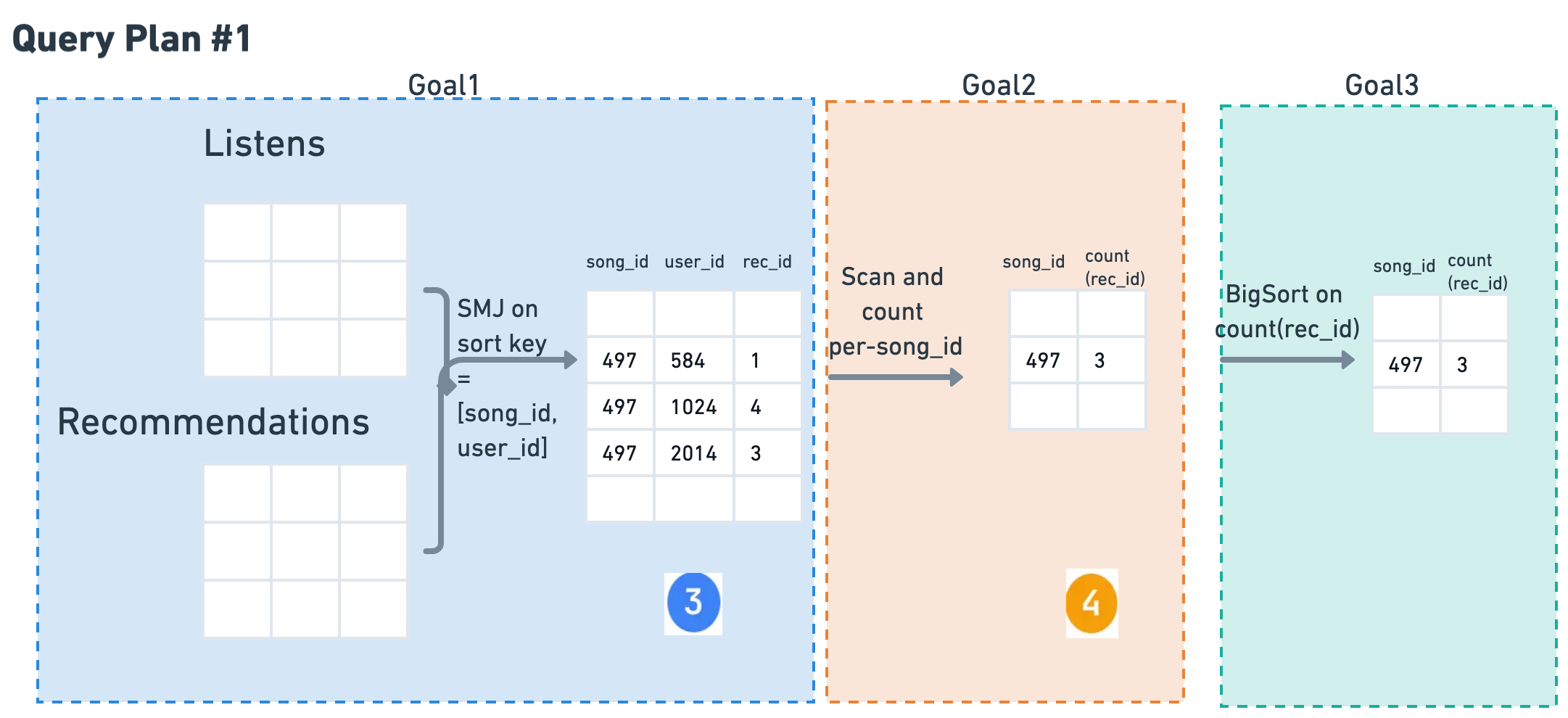
Query Plan 1: Sort-Merge Join, the three goals (Join, Group, Sort) with the what-happens and cost for each.

Figure 1. The query's three goals, left to right. Goal 1 (JOIN) sort-merge-joins Recommendations and Listens on (song_id, user_id), so the output is already sorted on both keys. Goal 2 (GROUP BY song_id) is then free: song_id is a prefix of that sort order, so grouping is direct, reading (3) and writing (4). Goal 3 (SORT) is one final BigSort(4) for ORDER BY count. The sorted join at Goal 1 (mint) makes Goal 2 free; the total is the sum of the three.

Goal	What happens	Cost
#1 Join R, L on `[song_id, user_id]`	Sort-Merge Join. Output already sorted on both keys	`SMJ(R, L)`
#2 Group `BY song_id`	`song_id` is a prefix of the sort order, so we can group directly. Read `(3)`, write `(4)`	`C_r·P(3) + C_w·P(4)`
#3 Sort `ORDER BY count`	One final external sort of the grouped table `(4)`	`BigSort(4)`

Total cost (Plan #1): SMJ(R,L) + C_r·P(3) + C_w·P(4) + BigSort(4)

Query Plan #2: Hash-Partition Join

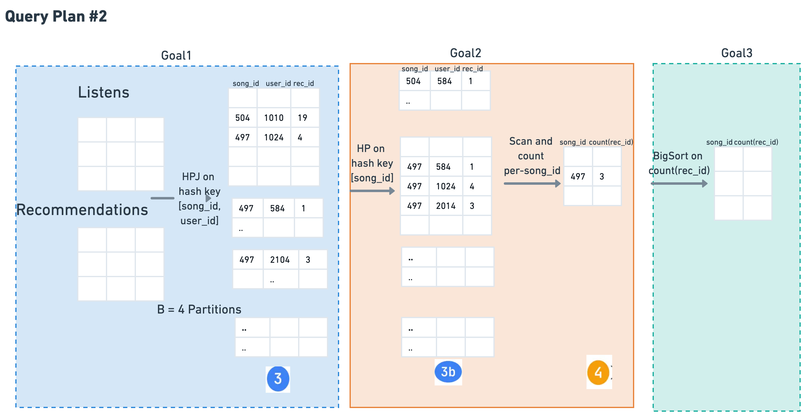
Query Plan 2: Hash-Partition Join, the three goals (Join, Group, Sort) with the what-happens and cost for each, including the extra re-partition before grouping.

Figure 2. The same three goals, left to right. Goal 1 (JOIN) hash-partition-joins on (song_id, user_id), so the output (3) is split on both keys. Goal 2 (GROUP BY song_id) is where Plan 2 pays: GROUP BY needs song_id alone, so (3) must be re-partitioned into (3b) before grouping, then read (3b) and write (4). That extra HP(3) step (mint) is the whole reason Plan 2 can cost more than Plan 1. Goal 3 (SORT) is the same final BigSort(4) as Plan 1.

Note. HPJ partitions on [song_id, user_id], so the output partitions (3) are split on both keys. Since GROUP BY is on song_id alone, we must re-partition (3) on song_id to align before grouping. That's the extra HP(3) step.

Goal	What happens	Cost
#1 Join R, L on `[song_id, user_id]`	Hash-Partition Join	`HPJ(R, L)`
#2 Group `BY song_id`	Re-partition `(3)` on `song_id` alone (call it `(3b)`); read `(3b)`, write `(4)`	`HP(3) + C_r·P(3b) + C_w·P(4)`
#3 Sort `ORDER BY count`	Final sort of `(4)`	`BigSort(4)`

Total cost (Plan #2): HPJ(R,L) + HP(3) + C_r·P(3b) + C_w·P(4) + BigSort(4)

Why the Plans Differ

Plan	Key property	Trade-off
Plan #1 (SMJ)	SMJ output is naturally sorted on the join keys; `song_id` is a prefix → can group directly	Pays the sort cost upfront via BigSort inside SMJ
Plan #2 (HPJ)	HPJ partitions on the join keys but `GROUP BY` needs only `song_id` → extra repartition step	Cheaper join when nothing is sorted, but pays repartitioning later

Both plans need a final BigSort for ORDER BY count. That's unavoidable because the output of grouping is in (song_id, count) order, not count order.

When to pick which

Choose SMJ when…	Choose HPJ when…
Data is pre-sorted or easily sortable	Data is unsorted and very large
Memory holds sort buffers	Hash partitioning is more efficient
Join keys align with `GROUP BY` keys	You can absorb the repartition cost

Next: Reading What a Real Optimizer Chose

So far we've estimated costs ourselves by writing out formulas. In practice, real databases do this work for you and show you the result via the EXPLAIN command. The Reading PostgreSQL EXPLAIN page takes the same cost-formula vocabulary and applies it the other way around: it decodes what plan a real optimizer picked, plus an interactive Colab for exploring plans.