Case Study 2.2: How OpenAI and Facebook Speed Up Queries with Vector Databases
Concept. A vector database indexes high-dimensional embeddings (typically 1,536-D) so "find the 10 most similar items" runs in milliseconds across millions of rows instead of comparing your query against every row.
Intuition. Embeddings turn meaning into coordinates, similar sentences sit near each other in 1,536-dimensional space. Without an index, finding the 10 most similar items requires comparing your query against every row. A vector database keeps a "what's near here?" index and answers in milliseconds.
Why Vector Databases
Objective: Understand approximate indices for high-dimensional data
When you're dealing with high-dimensional data, finding Approximate Nearest Neighbors (ANNs) is essential. OpenAI, for instance, uses text embeddings to sift through semantic layers across billions of documents. Traditional hashing methods simply don't make the cut.
Vector Databases: The Machine Behind Modern AI
Vector databases are engineered to handle high-dimensional vectors, like those from OpenAI's embeddings. They efficiently execute similarity searches in complex dimensional spaces using ANN algorithms.
FAISS: Facebook's Workhorse
FAISS is the library of choice for fast similarity search and clustering of dense vectors.
- Hardware: It uses GPUs to manage the indexing and searching, tasks that would otherwise overwhelm a CPU.
Example: Navigating a 768-Dimensional Maze
Consider a text embedding as a 768-dimensional vector, courtesy of Sentence-BERT. You can experiment with your own embeddings in FAISS via this Colab.
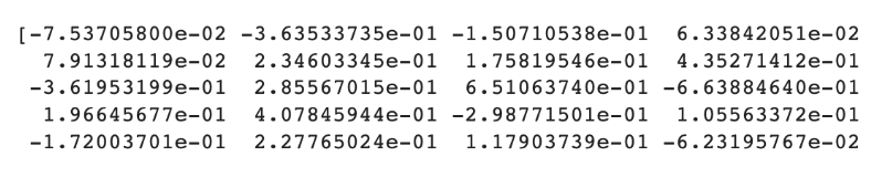
Example of a 768-dimensional text embedding vector
Here's how it works: embed 1000 strings into FAISS's vector index, then query for three strings to find their approximate nearest neighbors.
import faiss
FROM sentence_transformers import SentenceTransformer

# 768-D embeddings via Sentence-BERT
model = SentenceTransformer('all-mpnet-base-v2')
strings = [f"String {i}" for i IN range(1000)]
strings[42] = "String 42 IS making me hungry"
embeddings = model.encode(strings).astype('float32')

# Build a FAISS flat index OVER the 768-D vectors
index = faiss.IndexFlatL2(768)
index.add(embeddings)

# Query 3 strings, ask for top-5 nearest neighbors
queries = ["String 42",
           "String 42 IS making me hungry",
           "String 42 IS making me thirsty"]
query_emb = model.encode(queries).astype('float32')
distances, indices = index.search(query_emb, k=5)

for q, idx_row, dist_row IN zip(queries, indices, distances):
    print(f"Query: {q!r}")
    for i, d IN zip(idx_row, dist_row):
        print(f"  -> {strings[i]!r}  (distance {d:.3f})")
Search Results:
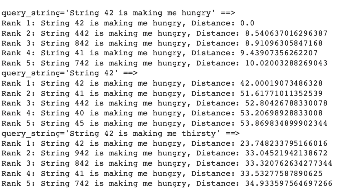
FAISS Nearest Neighbor output
Notice how "String 42 is making me hungry" finds an exact match (Distance: 0.0). It also pulls in related strings in this 768-dimensional space. Meanwhile, “String 42” and “String 42 is making me thirsty” find similar strings, though not exact matches.
Locality Sensitive Hashing (LSH): The Speed Specialist
LSH offers a speed boost by trading off some accuracy. Test out Vector Search and LSH in this Hashing Colab.
In this setup, the IndexLSH object is trained on a dataset and used to find approximate nearest neighbors for a new query point.
import faiss
FROM sentence_transformers import SentenceTransformer

# Same 1000 strings, same 768-D Sentence-BERT embeddings
model = SentenceTransformer('all-mpnet-base-v2')
embeddings = model.encode(strings).astype('float32')

# Build an LSH index. nbits = number of random hyperplanes:
# more bits give finer buckets but slower lookup.
d, nbits = 768, 64
index_lsh = faiss.IndexLSH(d, nbits)
index_lsh.train(embeddings)   # learns the random projections
index_lsh.add(embeddings)     # hashes each vector INTO buckets

# Approximate nearest-neighbor search for a query
query = model.encode(["String 42 IS making me hungry"]).astype('float32')
distances, indices = index_lsh.search(query, k=5)

for i, dist IN zip(indices[0], distances[0]):
    print(f"  -> {strings[i]!r}  (Hamming distance {dist})")
The IndexLSH object, once trained, identifies approximate nearest neighbors by clustering vectors that land on the same side of random planes.
Standard Hashing vs. LSH: A Quick Comparison
| Feature | Standard Hashing | Locality Sensitive Hashing |
|---|---|---|
| Goal | Avoid collisions (Unique buckets) | Encourage collisions (Similar items together) |
| Logic | Small input change → Massive hash change | Small input change → Small/No hash change |
| Usage | Exact lookups, Join partitioning | Similarity search, Recommendation engines |
Bottom Line: LSH adapts traditional indexing to manage the complexity of high-dimensional AI data, enabling us to search for "closeness" instead of mere "equality."