Microschedules: Deconstructing Concurrent Transactions
Concept. A microschedule is a precise, time-ordered interleaving of every atomic operation (Read, Write, Lock-request, Lock-grant, Unlock) from concurrent transactions, exposing exactly which operation runs when.
Intuition. Mickey's Req(L1) → Get(L1) → R(L1) → W(L1) → Unl(L1) and Minnie's Req(L1) → Get(L1) → R(L1) → W(L1) → Unl(L1) interleave step-by-step in the microschedule, making it visible whether Minnie's request blocks behind Mickey's grant or whether they conflict at all.
How to Build a Microschedule
1. Decompose Into Actions
Break down each transaction into atomic operations using a lock protocol.
Lock Pattern: Req→Get→[R/W]Unl
T1: Req(A)→Get(A)→R(A)→W(A)→Unl(A)
T2: Req(B)→Get(B)→R(B)→W(B)→Unl(B)
2. Interleave for Speed
Mix actions from different transactions to maximize CPU efficiency.
Smart: While T1 waits for IO, run T2
Result: 31 units (interleaved) vs 48 units (serial)
35% speedup from overlapping operations!
3. Track Dependencies
Construct a WaitsFor graph to ensure correctness.
Graph: T1→T2 = T1 waits for T2's lock
Safety: No cycles = No deadlock ✓
Action: Detect & resolve if cycles appear
Example 1: Serial Schedule (S1)
Serial Schedule with T3 → T2 → T1
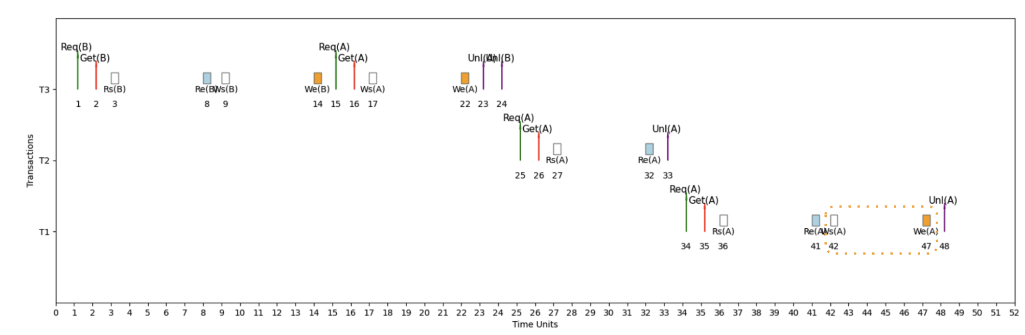
Here's an example micro schedule for S1, our serial schedule with T3 → T2 → T1, with completion = 48 units.
How to Read This Timeline
The Setup: 3 Transactions (T1, T2, T3) on 1 CPU Core
Time flows left → right, each transaction gets its own horizontal lane.
The Lock Pattern: Req → Get → [IO] → Unl
- Req = Request lock
- Get = Lock granted
- IO = Rs/Re or Ws/We
- Unl = Unlock (or Release)
Why This Matters: With 1 core for 3 transactions, the CPU constantly switches - when T1 waits for IO, T2 runs; when T2 waits for a lock, T3 runs. This interleaving maximizes CPU usage!
WaitsFor Graph: Detecting Deadlocks
Definitions
WaitsFor Graph
A directed graph representing lock dependencies between transactions in a concurrent execution schedule.
Components:
• Each node corresponds to a transaction
• Directed edges indicate waiting relationships
• Labels show the variable and time span of waiting
⚠ Deadlock Detection
Cycles within the WaitsFor graph signify deadlock.
Example: T1 waits for T2, T2 waits for T1 → Cycle = Deadlock
Impact of Deadlocks
Deadlocks can cause system stalls, leading to inefficiencies in resource utilization and transaction delays.
Consequences:
• System becomes unresponsive
• Transactions cannot proceed
• Manual intervention required
Example 2: Interleaved Schedule (S2) - Fast Execution
Interleaved Schedule with Optimized Performance
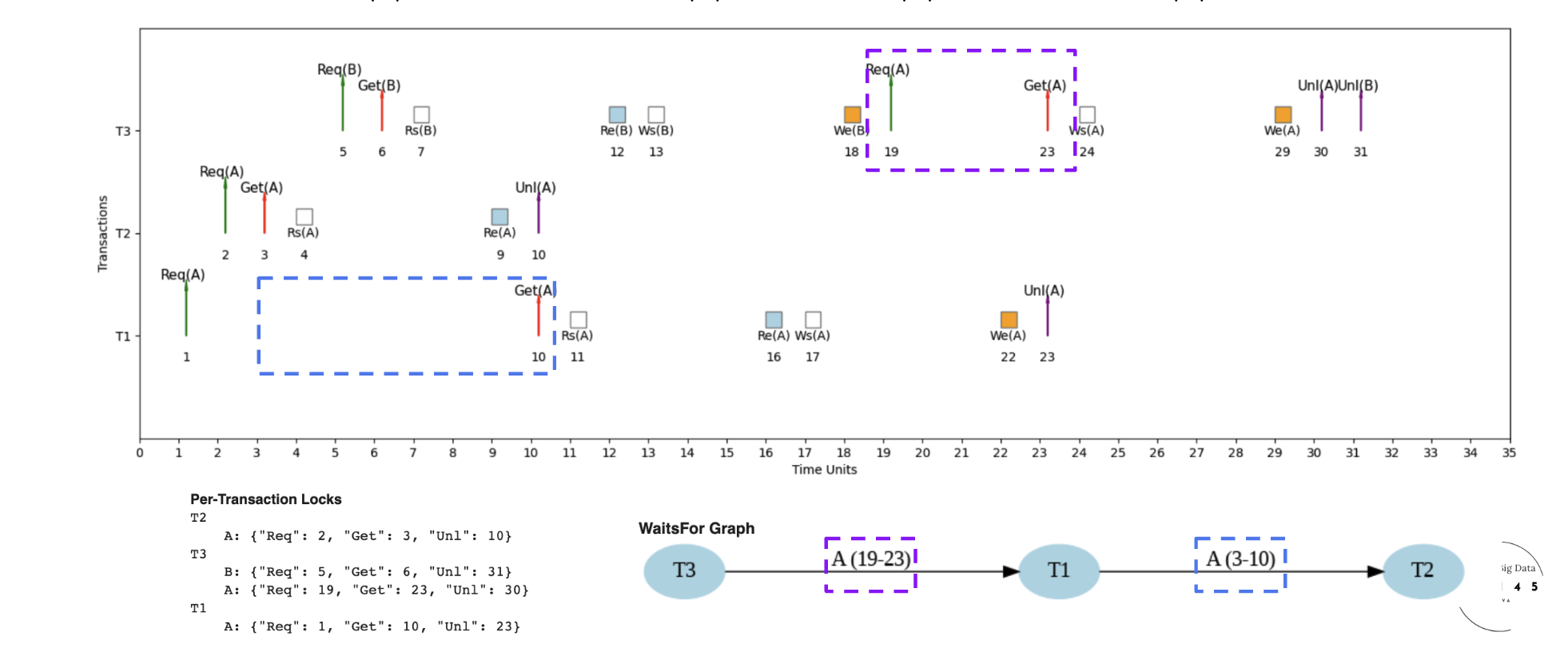
Here's an example micro schedule for S2, our interleaved schedule, with completion = 31 units.
Lock sequence: T2 takes lock A at unit 3, releases at 10; T1 then waits and acquires A at 10. The WaitsFor graph has one edge T1 → T2. No cycles, no deadlock.
Example 3: Interleaved Schedule (S3) - Different Microschedule
Different Interleaved Schedule for Same Transactions
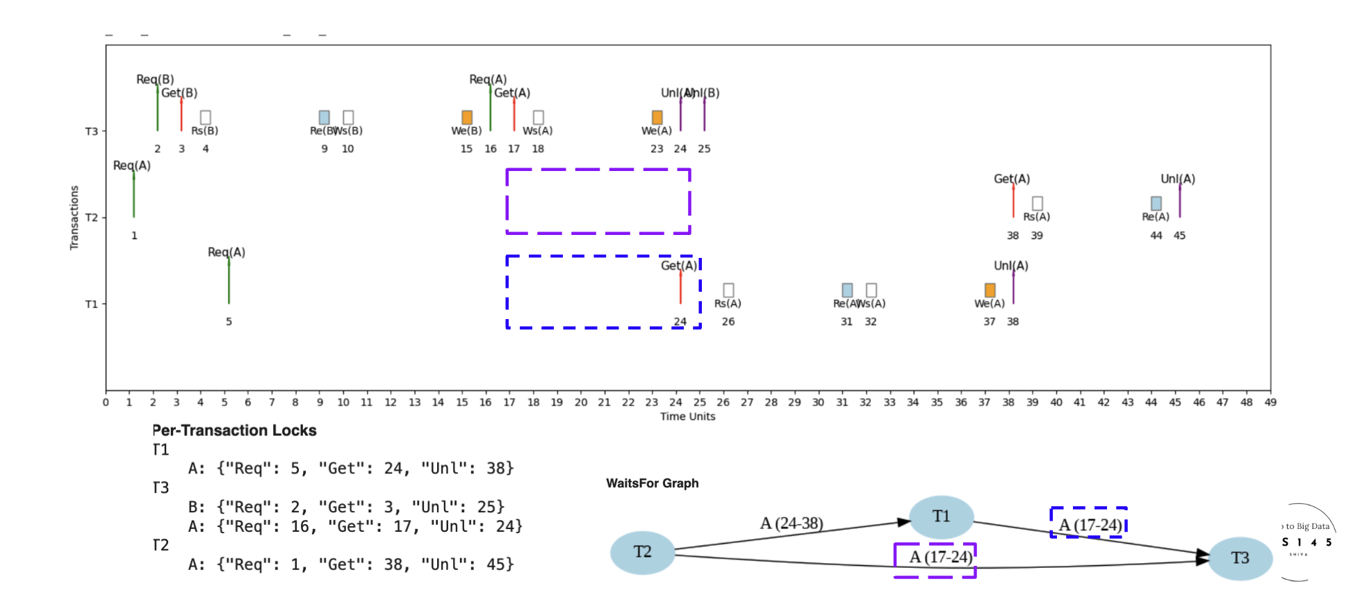
Here's an example micro schedule for S3, a different interleaved schedule for the same set of transactions, with completion = 45 units.
S3 vs S2: same three transactions, different lock-acquisition order produces more contention and longer waits. 45 units vs S2's 31. The scheduler's choices matter as much as the transactions themselves.
Example 4: Deadlock Detection
When Cycles Create System Deadlock
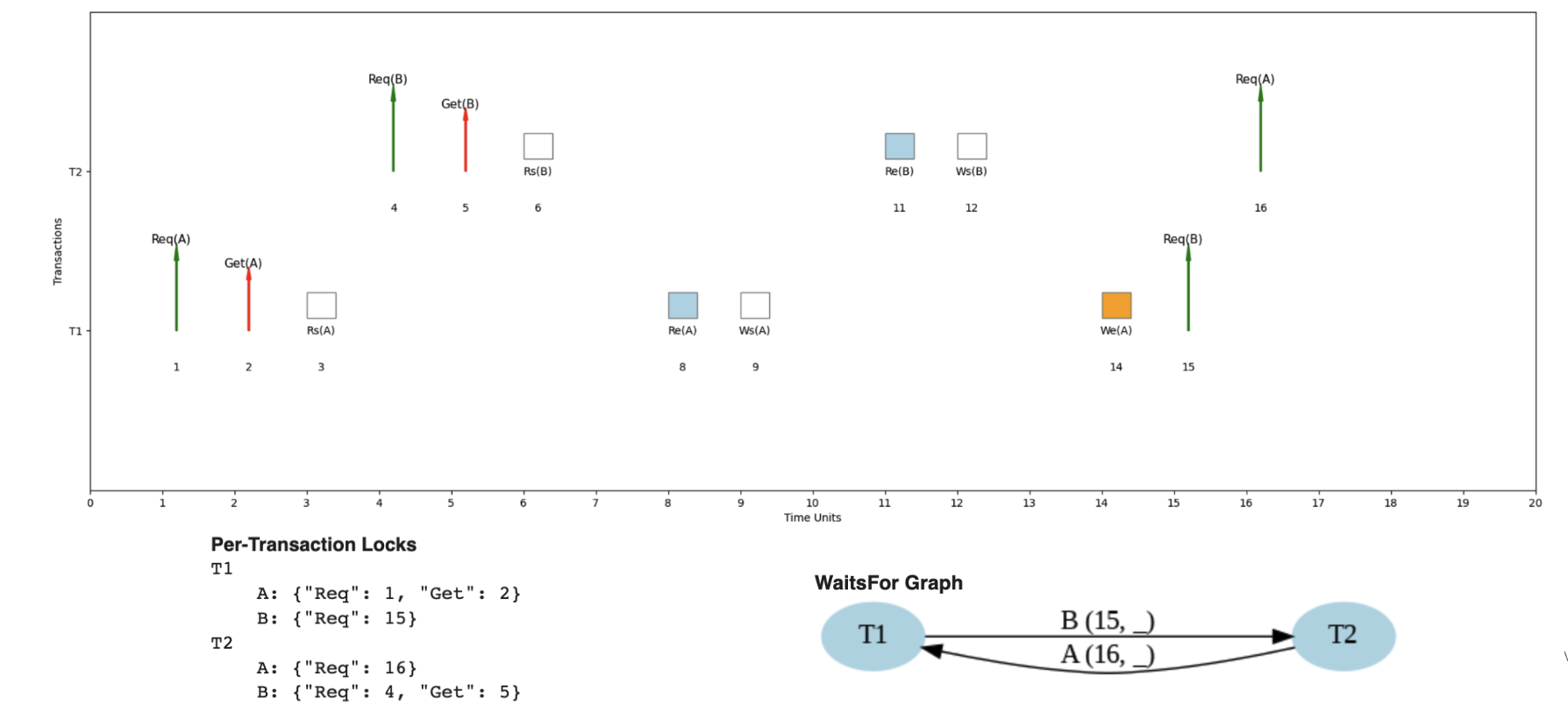
Here's an example where the same transaction pattern could lead to deadlock under different timing.
Circular wait: T1 waits for T2 to release B; T2 waits for T1 to release A. The WaitsFor graph has the cycle T1 → T2 → T1. Neither can proceed. Probability rises with more concurrent transactions; the database needs an explicit deadlock-detection-and-resolution mechanism.
Performance: Why Interleaved Schedules Win
The Power of Overlapping CPU and IO
| # of Transactions | IOlag | Serial Time | Interleaved Time | Speedup |
|---|---|---|---|---|
| 10 | 5 | 135 | 68 | 1.99× |
| 10 | 10 | 225 | 76 | 2.96× |
| 10 | 100 | 1,845 | 229 | 8.06× |
| 100 | 5 | 1,485 | 698 | 2.13× |
| 100 | 10 | 2,475 | 704 | 3.52× |
| 100 | 100 | 20,295 | 825 | 24.6× |
The bottom row is the dramatic case: with 100 transactions and IOlag = 100, interleaving wins by 24×.
Interleaved schedules provide significant advantages over serial schedules through smart resource utilization. The core idea is to overlap operations: CPU runs T2 while T1 waits for IO, and so on. The bigger the IO lag and the more concurrent transactions in flight, the bigger the win.
Concrete numbers: with 100 concurrent transactions and an IO lag of 100 time units, serial execution costs 10,000 units while interleaved finishes in ~417. A 24× speedup.