IO Cost Summary: Comparing Query Plans

The Query

-- Highly recommended songs
SELECT r.song_id, COUNT(r.recommendation_id) AS recommendation_count
FROM Recommendations AS r
JOIN Listens AS l ON r.user_id = l.user_id AND r.song_id = l.song_id
GROUP BY r.song_id
ORDER BY COUNT(r.recommendation_id) DESC;

Query Plan #1: Sort-Merge Join

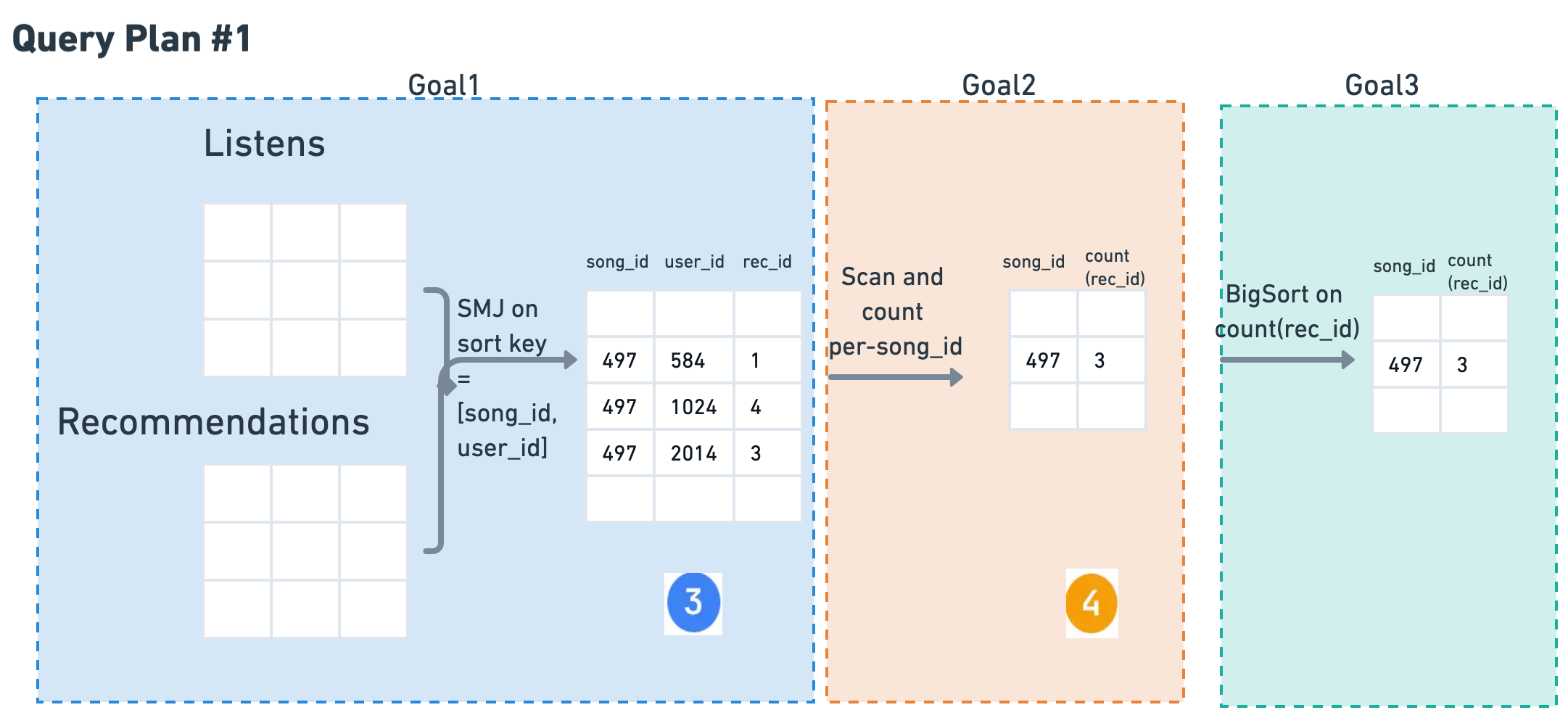
Goal #1: Join

Join R and L on

[song_id, user_id]

Cost: SMJ(R, L)

Goal #2: Group

GROUP BY song_id

Read 3, Write 4

Cost: C_r×P(3) + C_w×P(4)

Goal #3: Sort

ORDER BY count

Sort table 4

Cost: BigSort(4)

Total Cost of Plan #1:

SMJ(R, L) + C_r×P(3) + C_w×P(4) + BigSort(4)

Query Plan #2: Hash-Partition Join

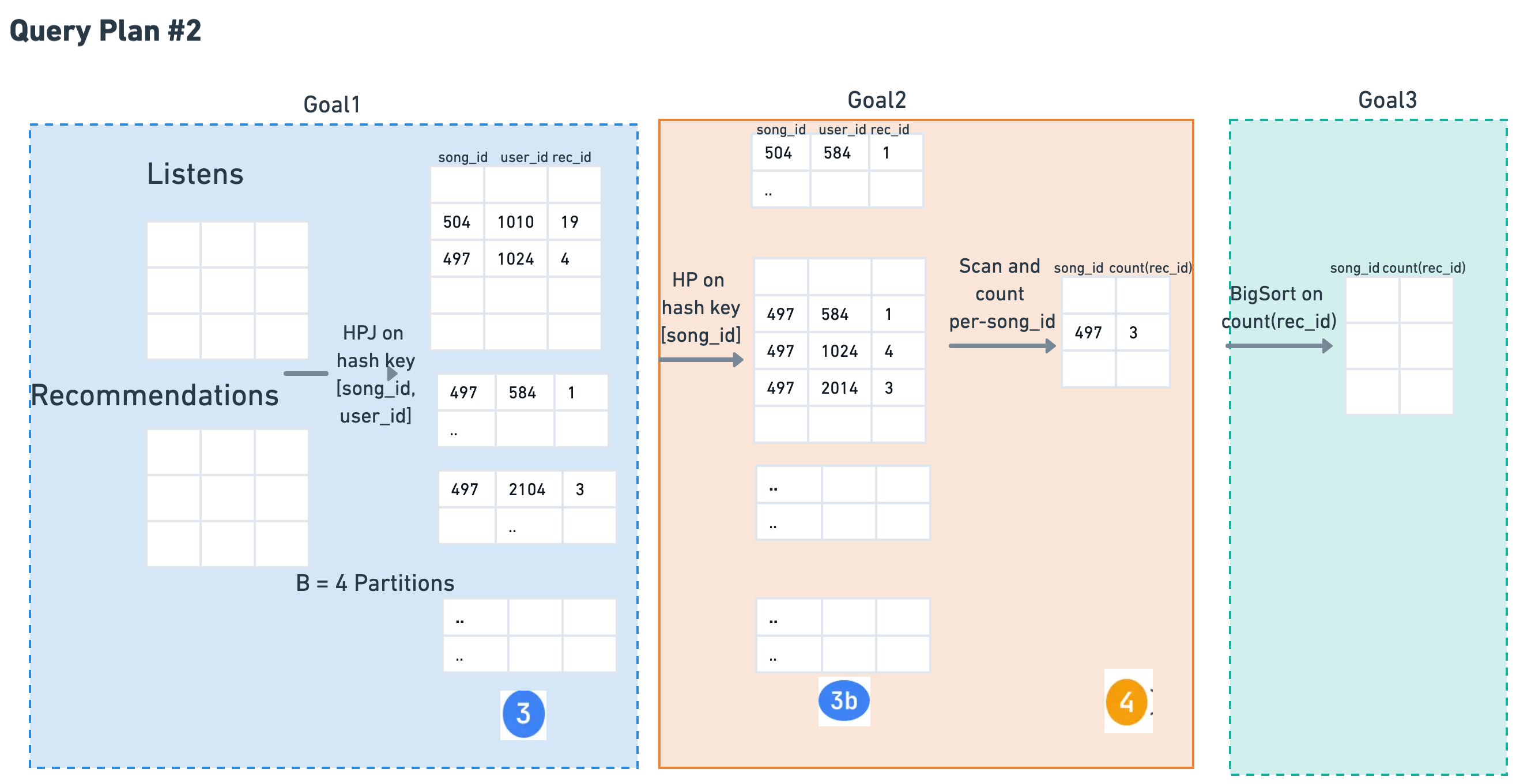
⚠️ Note: HPJ is on [song_id, user_id], so the output partitions (table ③) are based on both keys. Since GROUP BY is only on song_id, we need a second HP operation to repartition by song_id alone.

Goal #1: Join

Hash-Partition Join

[song_id, user_id]

Cost: HPJ(R, L)

Goal #2: Group

GROUP BY song_id only

HP on song_id to align partitions

HP 3, Read 3b, Write 4

Cost: HP(3)+C_r×P(3b)+C_w×P(4)

Goal #3: Sort

ORDER BY count

Sort table 4

Cost: BigSort(4)

Total Cost of Plan #2:

HPJ(R, L) + HP(3) + C_r×P(3b) + C_w×P(4) + BigSort(4)

Key Insights: Understanding the Query Plans

🔑 Why Different Sequences?

Plan #1: SMJ Approach

SMJ produces sorted output on join keys
Output already sorted by [song_id, user_id]
Can directly GROUP BY song_id (prefix key)
Only needs final BigSort for ORDER BY

Plan #2: HPJ Approach

HPJ partitions on both [song_id, user_id]
But GROUP BY needs only song_id
Must repartition (HP) to align with GROUP BY
Still needs BigSort for final ORDER BY

📌 Critical Observations

Always check join keys vs GROUP BY keys: Mismatch requires repartitioning
HP twice in Plan #2: First for join (both keys), second for grouping (single key)
Both plans need final sort: ORDER BY count requires BigSort regardless
Trade-off: SMJ has sort overhead upfront, HPJ has partition overhead midway

When to Use Which?

Choose SMJ when...	Choose HPJ when...
• Data is pre-sorted or easily sortable • Memory can hold sort buffers • Join keys align with GROUP BY keys	• Data is unsorted and very large • Hash partitioning is more efficient • Willing to pay repartition cost

Interactive Query Explainer

Colab for Query Optimizer

Example #3: The Optimizer's Choice

The Final Query Plan: What PostgreSQL Actually Chose

-- Popular songs based on number of listens
SELECT Songs.title, Songs.artist, COUNT(Listens.song_id) AS popular
FROM Songs
JOIN Listens ON Songs.song_id = Listens.song_id
GROUP BY Songs.title, Songs.artist
ORDER BY COUNT(Listens.song_id) DESC
LIMIT 10;

EXPLAIN Output

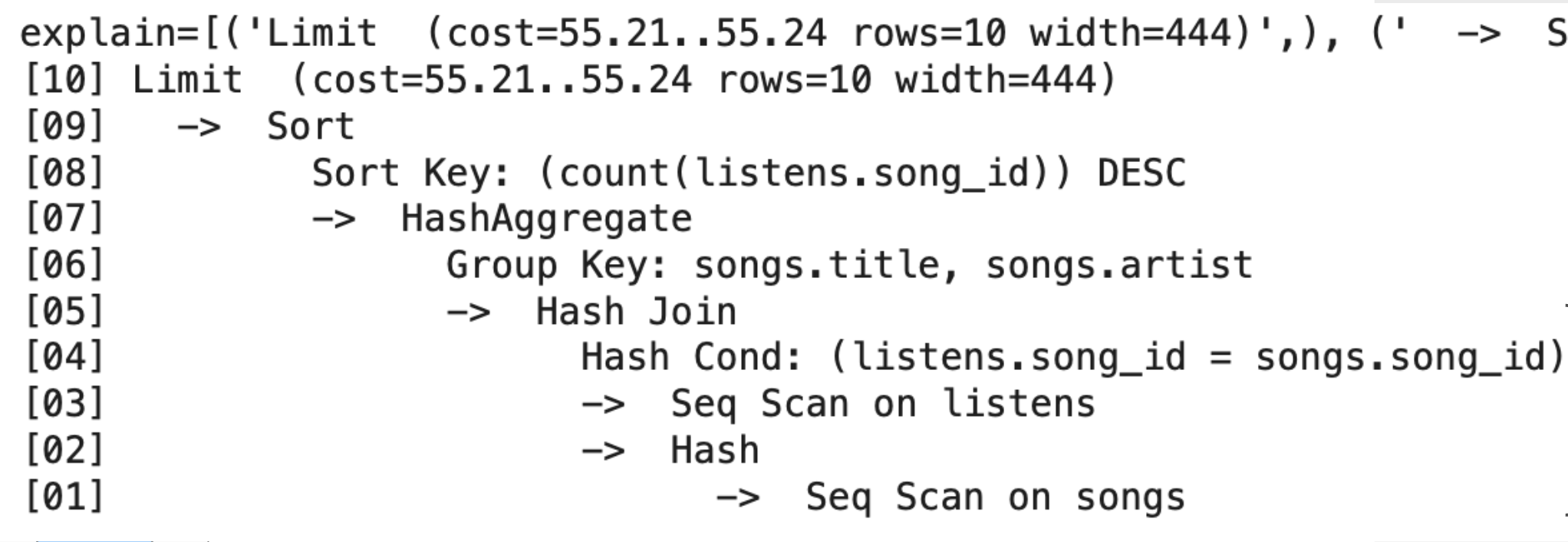
How to Read EXPLAIN and Calculate Costs

📖 Read Bottom-Up (Innermost First)

Cost Format

cost=startup..total

startup: Cost before first row
total: Cost for all rows
rows: Estimated row count

Step-by-Step Cost Calculation

[01] Seq Scan on songs
C_r × P(Songs) = Read base table
[02-03] Build Hash + Seq Scan listens
C_r × P(Listens) = Read second table
[04-05] Hash Join
HPJ(Songs, Listens) on song_id
[06-07] HashAggregate
HashAgg for GROUP BY (no sort needed!)
[08-09] Sort
BigSort for ORDER BY count
[10] Limit
Negligible cost (just take 10 rows)

Mapping to Our IO Cost Formulas

PostgreSQL Operation	Our Formula	Cost
Seq Scan (×2)	`C_r × P(Songs) + C_r × P(Listens)`	Base scans
Hash Join	`HPJ(Songs, Listens)`	Join cost
HashAggregate	`Grouping cost`	Aggregation
Sort	`BigSort(grouped_data)`	Sorting
Total	Sum of all operations	55.24 units

Understanding HashAggregate

HashAgg builds an in-memory hash table:

Input: Full table scan
Output: One row per group (usually much smaller!)
IO Cost: C_r×P(input) - no sorting needed
If spills: Becomes partition-based like HPJ

💡 Why Did PostgreSQL Choose This Plan?

Hash Join chosen: More efficient than SMJ for unsorted data
HashAggregate used: Can group without sorting (unlike our simplified model)
Only one BigSort: Just for the final ORDER BY
Total cost 55.24: Optimizer estimated this as cheapest plan
Lesson: Real optimizers have more tricks (HashAgg vs sort-based grouping)

Common EXPLAIN Operations Reference

Operation	What it does	IO Cost	Output Rows	Output Size
HashAggregate	Groups using hash table	`C_r×P(input)`	One per group	≪ input
WindowAgg	ROW_NUMBER, RANK, etc	`C_r×P(input) + sort`	Same as input	Slightly larger (extra cols)
CTE Scan	Reads WITH result	`C_r×P(CTE)`	= CTE rows	= CTE size
Subquery Scan	Reads subquery	`C_r×P(subquery)`	= subquery rows	= subquery size
Index Scan	Uses index	`Log(N) + rows`	Filtered rows	≪ input
Bitmap Scan	Batch index reads	Better for many rows	Filtered rows	≪ input
Nested Loop	For each row, probe	`P(R) × P(S)` worst	Join matches	Varies
Hash Join	Build hash, probe	`P(R) + P(S)`	Join matches	Varies
Materialize	Cache in memory	`C_w + n×C_r`	Same as input	= input
Sort	Order rows	`BigSort` cost	Same as input	= input

🔑 Key Insight: WindowAgg keeps all rows but adds columns (rank, row_number), while HashAgg reduces to one row per group!