Microschedules: Deconstructing Concurrent Transactions
What is a Microschedule? 🔬
Key Concept: A microschedule is a specific execution sequence of atomic Read/Write (R/W) and Lock (Req/Get/Unlock) actions from concurrent transactions.
How to Build a Microschedule
1️⃣ Decompose Into Actions
Break each transaction into atomic operations with lock protocol
T1: Req(A)→Get(A)→R(A)→W(A)→Unl(A)
T2: Req(B)→Get(B)→R(B)→W(B)→Unl(B)
2️⃣ Interleave for Speed
Mix actions from different transactions to maximize CPU usage
Result: 31 units (interleaved) vs 48 units (serial)
35% speedup from overlapping operations!
3️⃣ Track Dependencies
Build WaitsFor graph to ensure correctness
Safety: No cycles = No deadlock ✓
Action: Detect & resolve if cycles appear
Example 1: Serial Schedule (S1) ⚙️
Serial Schedule with T3 → T2 → T1
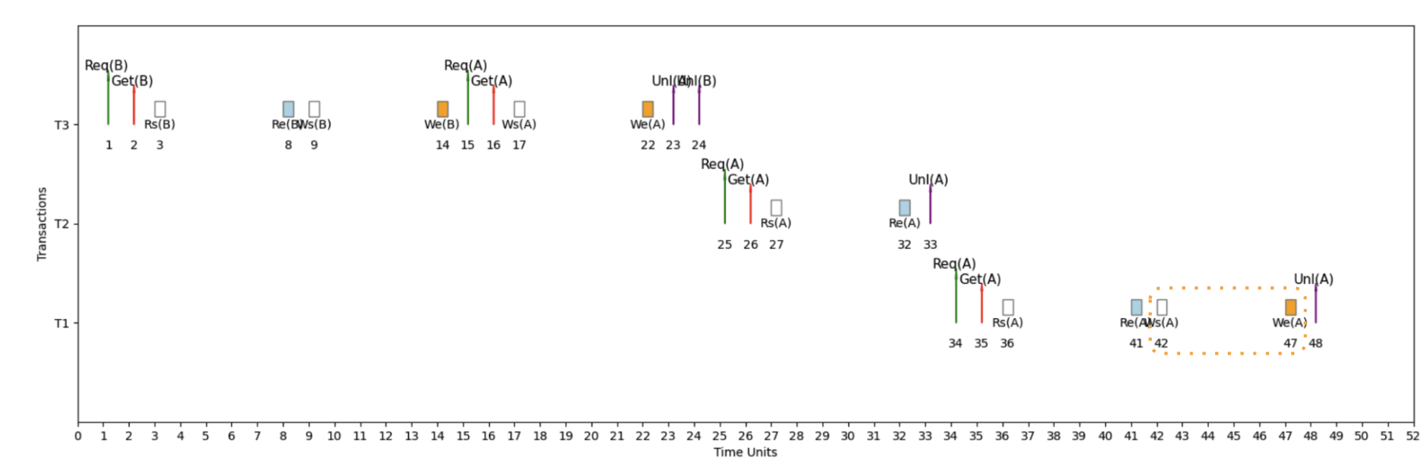
Here's an example micro schedule for S1, our serial schedule with T3 → T2 → T1, with completion = 48 units.
📖 How to Read This Timeline
Time flows left → right, each transaction gets its own horizontal lane
Req → Get → [IO] → Unl
- Req = Request lock
- Get = Lock granted
- IO = Rs/Re or Ws/We
- Unl = Unlock (or Release)
WaitsFor Graph: Detecting Deadlocks 🔍
Definitions
🔗 WaitsFor Graph
WaitsFor graph is a directed graph that represents the lock dependencies between transactions in a concurrent execution schedule.
• Each node corresponds to a transaction
• Directed edges indicate waiting relationships
• Labels show the variable and time span of waiting
⚠️ Deadlock Detection
Cycles within the WaitsFor graph signify deadlock.
💥 Impact of Deadlocks
Deadlocks can cause system stalls, leading to inefficiencies in resource utilization and transaction delays.
• System becomes unresponsive
• Transactions cannot proceed
• Manual intervention required
Example 2: Interleaved Schedule (S2) - Fast Execution 🚀
Interleaved Schedule with Optimized Performance
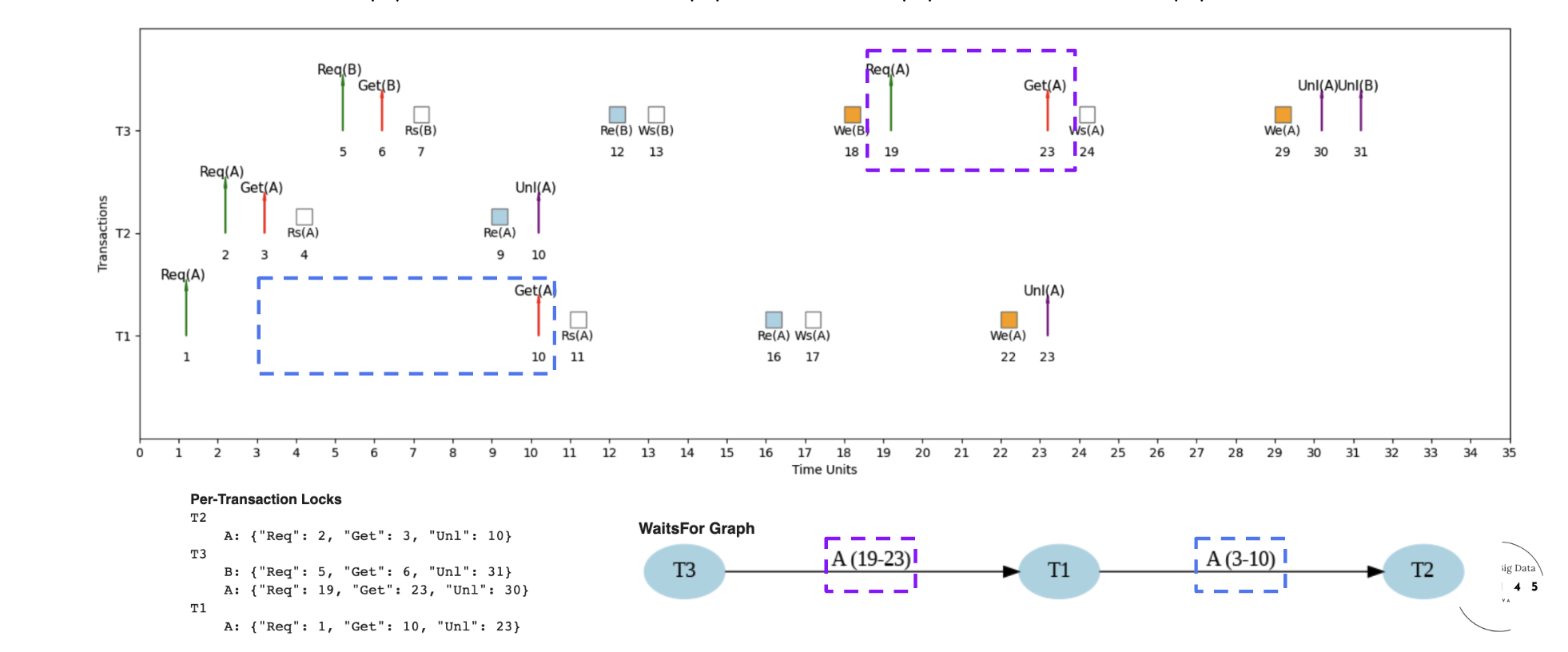
Here's an example micro schedule for S2, our interleaved schedule, with completion = 31 units.
📖 How to Read S2: Timeline, Locks & Dependencies
- Time flows left → right (0 to 31 units)
- Each row = one transaction (T1, T2, T3)
- T2: T2.Req(A) at 2, T2.Get(A) at 3, T2.Unl(A) at 10
- Note: T1.Get(A) waits for T2.Unl(A)
- Lock pattern determines execution order
- Nodes: T1, T2, T3 (transactions)
- Edge: T1→T2, T1 waits for T2 on variable A (time units 3-10)
- No cycles detected = No deadlock ✓
Example 3: Interleaved Schedule (S3) - Different Microschedule ⏱️
Different Interleaved Schedule for Same Transactions
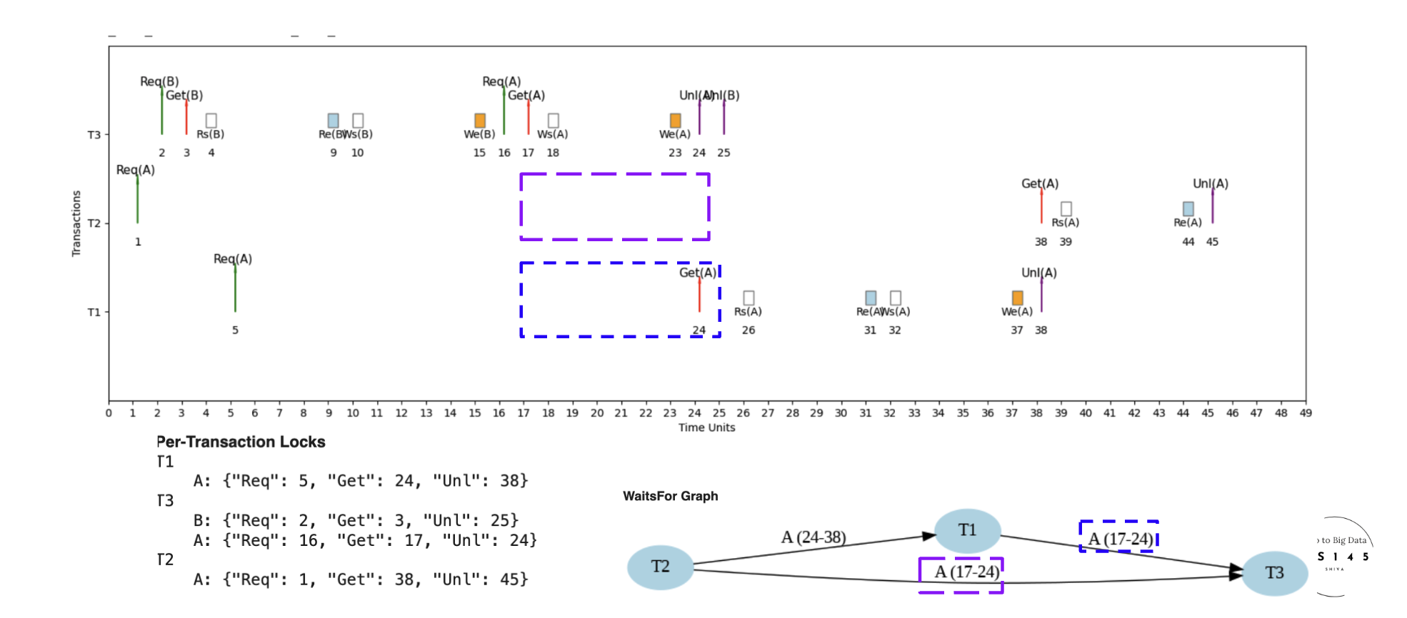
Here's an example micro schedule for S3, a different interleaved schedule for the same set of transactions, with completion = 45 units.
🔄 S3 vs S2: Different Microschedule, Same Transactions
S3 takes 45 units vs S2's 31 units due to different lock acquisition order and contention patterns
More contention leads to longer waits and slower completion - same transactions, different execution strategy
Same transactions can have vastly different performance based on microschedule scheduling decisions!
Example 4: Deadlock Detection ⚠️
When Cycles Create System Deadlock
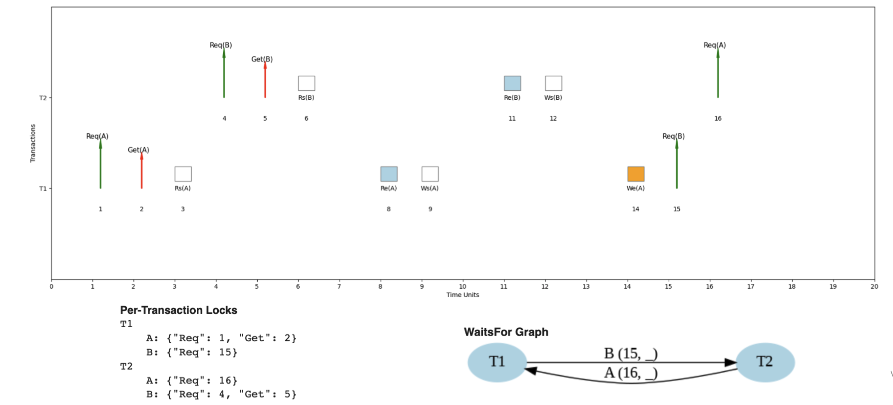
Here's an example where the same transaction pattern could lead to deadlock under different timing.
💥 Understanding Deadlock Scenarios
- T1 waits for T2 to release resource B
- T2 waits for T1 to release resource A
- Result: Circular wait = Deadlock!
- T1 → T2 → T1 (cycle detected)
- Each arrow represents a "waits for" relationship
- Cycle means no transaction can proceed
- System requires deadlock detection & resolution
- Can occur with 2+ transactions
- More likely with ≥3 transactions due to dependencies
- Probability increases with more concurrent transactions
- Prevention: careful resource ordering
Performance: Why Interleaved Schedules Win 🚀
The Power of Overlapping CPU and IO
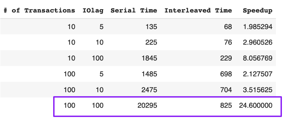
Interleaved schedules provide significant advantages over serial schedules through smart resource utilization.
⚡ Speedup Analysis: CPU + IO Optimization
- CPU operations run while waiting for IO completion
- No idle CPU time during disk/network waits
- Multiple transactions progress simultaneously
- Maximum resource utilization achieved
- Serial: T1 complete → T2 complete → T3 complete
- Interleaved: T1, T2, T3 run concurrently
- Higher IO lag = bigger speedup opportunity
- More concurrent transactions = greater parallelism
- 100 concurrent transactions
- IO lag: 100 time units
- Result: 24x speedup!
- Serial: 10,000 units vs Interleaved: 417 units